Triple-barrier labeling¶

The labeling problem from the previous lesson requires that events occur at specific times, labels respect path dependence, and magnitudes be comparable across regimes. Triple-barrier is the procedure that satisfies all three requirements.

The procedure is a few lines of code with significant pedagogical depth.

Three barriers, one label¶

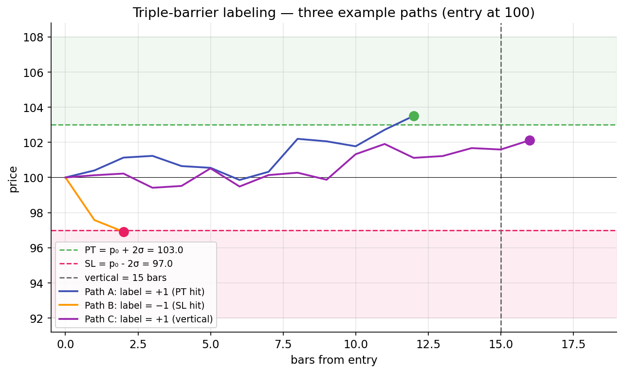
At each event at time $t_0$, draw three barriers:

Upper barrier at price $p_0 \cdot (1 + \text{pt\_mult} \cdot \sigma)$ — a profit-take, set some multiple of current vol above entry.
Lower barrier at price $p_0 \cdot (1 - \text{sl\_mult} \cdot \sigma)$ — a stop-loss, same logic below.
Vertical barrier at time $t_0 + \text{vertical\_bars}$ — a time stop, always present to prevent infinite holds.

Walk forward from $t_0$ bar by bar. The first barrier the price touches determines the label:

Upper hit first → label $= +1$, barrier_hit = "pt".
Lower hit first → label $= -1$, barrier_hit = "sl".
Vertical reached first (neither barrier crossed) → label $= \text{sign}(r_\text{final})$, barrier_hit = "vertical".

The label is always in $\{-1, 0, +1\}$, with $0$ possible only at the vertical barrier with exactly zero net return (rare but permitted).

Three example paths from the same entry at p₀ = 100, σ = 1.5, with pt_mult = sl_mult = 2 and vertical = 15 bars. Path A hits the profit-take barrier and is labeled +1; Path B hits the stop-loss and is labeled −1; Path C drifts modestly upward and terminates at the vertical barrier, taking the sign of its net return.

Why vol-scaling matters¶

Barriers are scaled by a rolling vol target $\sigma$ rather than fixed dollar amounts. The upper barrier for an event at $t_0$ is $p_0 \cdot (1 + 2 \sigma_{t_0})$ when pt_mult = 2.0, where $\sigma_{t_0}$ is the volatility at entry.

The scaling serves two purposes:

Regime-comparable labels. The same pt_mult produces labels of comparable difficulty across regimes. In a low-vol regime ($\sigma = 0.5\%$), the 2σ barrier is at +1%. In a high-vol regime ($\sigma = 3\%$), the 2σ barrier is at +6%. A profit-take label of +1 answers the same question in both cases: did the move exceed noise by a material factor? The binary label is comparable across regimes.
Prevents pathological outcomes. A fixed dollar barrier (for example, always +$5) is hit almost immediately in high-vol regimes (nearly every event is a winner) and almost never in low-vol regimes (nearly every event times out). Neither extreme produces useful labels.

The rolling vol used is afml.labeling.rolling_vol: EWM standard deviation of arithmetic returns with span=100 by default. The choice of arithmetic over log returns is documented in Lesson 1 — barriers compare p_t / p_0 - 1 against mult * σ, requiring both quantities in arithmetic-return units.

The side adjustment¶

Triple-barrier handles both long and short primary signals through a side parameter.

For a long signal (side = +1), the return series is $p_t / p_0 - 1$. A rising price produces positive returns; the upper barrier (profit-take for a long) is hit when returns rise, and the lower barrier (stop-loss) is hit when they fall.

For a short signal (side = -1), the return series is multiplied by the side: $(p_t / p_0 - 1) \cdot \text{side} = -(p_t / p_0 - 1)$. A rising price now produces negative side-adjusted returns, correctly representing a losing short. The upper barrier — still the profit-take — is hit when the side-adjusted return rises, which occurs when the underlying falls.

The output label uses the same sign convention regardless of side: $+1$ indicates a profitable trade, $-1$ indicates an unprofitable one. A profitable long receives label $+1$; a profitable short also receives label $+1$. The sign reflects trade profitability, not price direction.

Vertical barrier: edge cases¶

The vertical barrier caps the holding period. Without it, an event might never hit either horizontal barrier in bounded time, and the labeling loop would be unbounded. The vertical barrier is typically set to 5-20 bars for daily data, depending on the strategy's target horizon.

The edge case occurs at the vertical barrier itself. If the vertical is reached with positive realized return but no upper-barrier hit, the label is $\text{sign}(\text{return}) = +1$. This captures the case where the trade was directionally correct but did not reach the profit-take threshold — still informative, labeled as a profit-take.

The label = sign(final_return) convention follows AFML. An alternative — label = 0 at vertical — is cleaner in the sense that no barrier was crossed but discards directional information. The signed convention preserves more information at the cost of slight interpretive ambiguity.

Output schema¶

The output of apply_triple_barrier is a DataFrame with the following columns:

Column	Type	Meaning
`event_idx`	Int64	Index of the event entry bar
`exit_idx`	Int64	Index at which a barrier was hit (or vertical reached)
`ret`	Float64	Side-adjusted realized return `(p_exit/p_entry - 1) * side`
`label`	Int8	`+1`, `0`, or `-1` per the rules above
`barrier_hit`	Utf8	`"pt"`, `"sl"`, or `"vertical"`

Each event produces a single row. The exit_idx is essential for computing the label horizon $t_1[i]$ used in purged-k-fold CV; without it, the model-selection step cannot determine the purge extent.

Tuning pt_mult and sl_mult¶

The two multipliers are the primary calibration parameters. Typical starting values are pt_mult = sl_mult = 2.0 (symmetric 2σ barriers). Variations:

Asymmetric barriers reflect asymmetric risk preferences. A "let winners run" strategy uses pt_mult > sl_mult (wider profit target, tighter stop). A mean-reversion strategy uses pt_mult < sl_mult (tight profit-take at the expected reversion, wider stop for overshoot).
Wider barriers produce fewer barrier hits (more vertical-barrier exits), slower label generation, and lower SNR per label.
Tighter barriers produce faster hits and more ±1 labels but also more whipsawing — moves that briefly cross a barrier before reversing generate labels that can be noisy.

Calibration should reflect the strategy's intended holding period and risk profile. A small grid over {1.5, 2.0, 2.5} for each multiplier is a reasonable starting scan.

Connection to primaries¶

Triple-barrier does not determine when to trade; it assigns a label to the outcome given an event. Events come from a primary signal:

RSI(2) crossing oversold/overbought (as in the capstone strategy).
Moving-average cross.
A GEX-regime flip.
A structural break detected by CUSUM.
A news-event trigger.

Events are generated externally and passed to apply_triple_barrier as bar indices. The function is agnostic to the rule that produced them, which keeps the primary swappable while the labeling remains universal.

Downstream uses of labels¶

Labels feed two downstream uses in the trading project:

Training a secondary model for meta-labeling (next lesson). The secondary's target is (label > 0) as a binary: did the primary's direction succeed? The meta_label function in afml.labeling binarizes the triple-barrier output.
Evaluating primaries. Before training a meta-labeler, raw primary performance can be analyzed descriptively from the triple-barrier output: what fraction of primary signals hit the upper barrier, what fraction hit the lower, how much of the return is captured.

Neither use is possible without labels. Neither is informative without sensible labels (not fixed-horizon returns).

Failure modes¶

Triple-barrier has its own failure modes:

Lagging vol scaling. The rolling_vol EWM uses a 100-day span. When the volatility regime shifts quickly, barriers may be calibrated to stale vol for several weeks, producing systematically miscalibrated labels.
Overlapping labels. As discussed in the labeling problem and purging lessons, consecutive events can produce overlapping label horizons. This is a cross-validation problem rather than a labeling problem per se, but it originates in the labeling construction.
Path ambiguity at barrier hits. When upper and lower barriers could both plausibly hit on the same bar (due to intrabar volatility), daily-bar data cannot disambiguate. The code uses bar-close prices; intraday paths may have crossed both barriers, but this is not visible in a daily labeling loop.

These failure modes are minor relative to the problems triple-barrier solves but should be considered when sanity-checking labels during high-volatility regimes.

Summary¶

The reader can now reason about:

Why a single apply_triple_barrier function handles both long and short signals: the side adjustment flips the return series, preserving consistent profit-take and stop-loss semantics.
Why vol-scaling produces labels comparable across regimes: a 2σ label carries the same meaning in 2017 and 2020 despite the dollar move differing by 5×.
The trade-offs in choosing pt_mult and sl_mult: tighter barriers produce more labels per unit time at the cost of noise; wider barriers produce slower but cleaner labels.

Implemented at¶

trading/packages/afml/src/afml/labeling.py:52 — apply_triple_barrier(prices, events, sides, config, vol):

events: array of integer indices identifying event bars.
sides: array of ±1 matching events; +1 for long, -1 for short.
config: BarrierConfig(pt_mult, sl_mult, vertical_bars).
vol: per-bar vol series (typically from rolling_vol).

The implementation loops over events, walking prices forward from each event until a barrier hits or vertical is reached. Label and exit index are recorded per event. The function has property tests and a known-value regression test per the AFML package's 90% coverage floor on labeling.

The meta_label(triple_barrier_out, sides) function at line 126 binarizes the output for secondary-model training: label > 0 → meta = 1, else meta = 0.

Next: Meta-labeling →