Delta — sensitivity to price
The Black-Scholes derivation produced a hedging portfolio \(\Pi = C - \Delta S\) whose first-order risk cancels. The coefficient \(\Delta\) — the partial derivative of option value with respect to the underlying — simultaneously describes exposure, hedge ratio, and an approximate probability of exercise.
Definition
Delta is the dollar change in an option's value per $1 change in the underlying. It is a rate evaluated at a specific \(S\), valid for small moves. For a European call under Black-Scholes:
so \(\Delta \in (0, 1)\). For a European put, by put-call parity:
so \(\Delta \in (-1, 0)\).
A call's price rises with the underlying, so its delta is positive. A put's price falls with the underlying, so its delta is negative. The magnitudes indicate how closely each option's value tracks the underlying.
Three regimes
Deep ITM: \(\Delta \to \pm 1\)
When a call's strike is well below the current spot and expiry is near, the option is nearly certain to finish ITM. Its value at expiry equals \(S_T - K\), which moves dollar-for-dollar with \(S_T\), so \(\partial V / \partial S\) approaches 1. A deep-ITM call behaves like stock net of a fixed obligation. Put-call parity confirms this algebraically: \(C = P + S - Ke^{-rT}\); when \(P\) is small (as in deep-ITM calls, which correspond to deep-OTM puts), \(\partial C / \partial S \approx 1\).
For a deep-ITM put, \(\Delta \to -1\), with the position moving inversely to stock.
Deep OTM: \(\Delta \to 0\)
When a call is far out of the money and near expiry, small moves in \(S\) have little effect on the probability of finishing ITM. The option value is dominated by the small time value of a low-probability event, and \(\partial V / \partial S\) approaches zero.
ATM: \(\Delta \approx 0.5\) for a call, slightly above
When \(S = K\) and sufficient time remains, the call has approximately a 50% risk-neutral probability of finishing ITM (via \(N(d_2)\)), and delta is approximately 0.5 — though not exactly. For a call with positive time to expiry and non-zero volatility, \(d_1 > d_2\), so \(N(d_1) > N(d_2)\). An ATM call's delta is typically in the 0.52–0.55 range. The offset reflects the asymmetry of upside versus downside payoffs: unbounded upside, bounded loss equal to the premium.
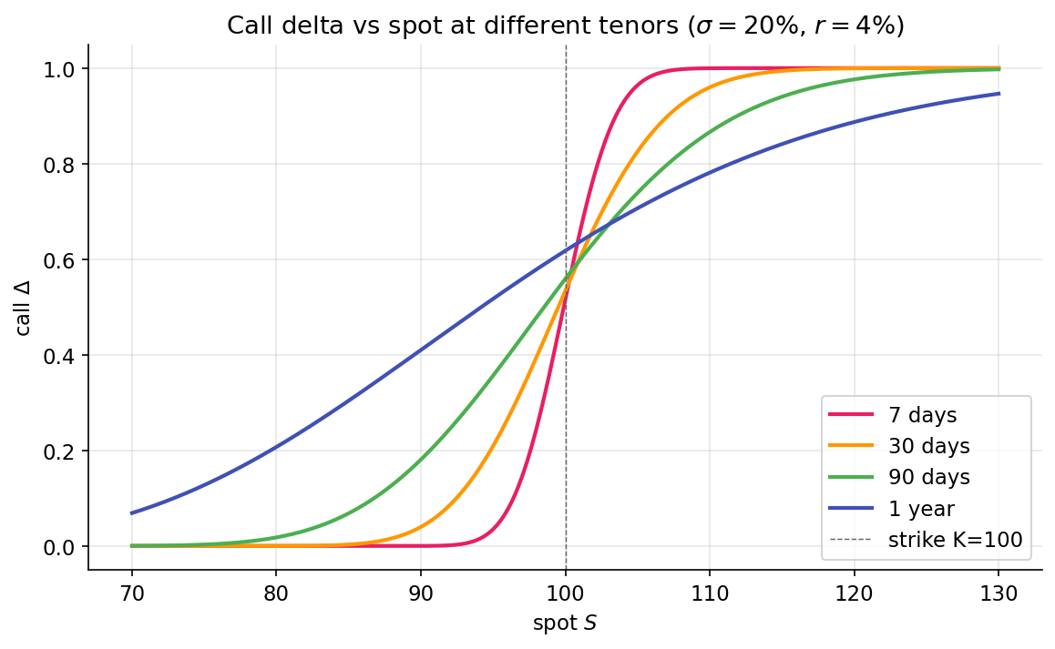
Across a range of spot values at several tenors, the three regimes form a single smooth S-curve whose slope at the strike sharpens as expiry shortens (7-day has the steepest transition; 1-year is diffuse):
Delta as hedge ratio
The Black-Scholes derivation produces this directly: the portfolio \(\Pi = C - \Delta S\) is locally riskless. A long call's exposure to the underlying equals that of \(\Delta\) long shares; shorting \(\Delta\) shares therefore neutralizes the first-order exposure.
Example: a position of 10 SPY calls with strike \(\$450\) and 30 days to expiry, with SPY at \(\$450\). Each contract covers 100 shares (the standard U.S. equity option multiplier). The call delta is 0.53 at these parameters.
- Position delta: \(10 \text{ contracts} \times 100 \text{ shares/contract} \times 0.53 = 530\) share-equivalents.
- Delta hedge: short 530 shares of SPY.
- Net position: approximately delta-neutral — portfolio P&L is near zero for small moves in SPY.
The term "delta-neutral" describes first-order neutrality, not overall profit neutrality. Second-order sensitivity (gamma, covered in the next lesson) remains, and theta (time decay) erodes value over time. The purpose of delta hedging is to isolate these second-order effects so they can be traded independently of directional exposure. Shorting shares against a long call removes directional exposure; what remains is a volatility position.
Delta as approximate probability
Traders often describe delta as the probability of finishing ITM. This is approximate. From the Black-Scholes formula:
\(\Delta\) equals the probability only in the limit of zero volatility or zero time. For a 30-day option with \(\sigma = 20\%\), \(\sigma \sqrt{T} \approx 0.058\), and the gap between \(N(d_1)\) and \(N(d_2)\) is small. For LEAPS (multi-year expiry), \(\sigma\sqrt{T}\) can exceed 0.4, and delta can overstate the exercise probability by several percentage points.
The "30-delta = 30% probability of ITM" shorthand is accurate enough for short-dated contracts. For long-dated positions, the distinction matters.
Delta-one products
Instruments that move one-for-one with the underlying have \(\Delta = 1\). The underlying itself satisfies this trivially. Futures approximately do (subject to cost-of-carry adjustments); ETFs tracking the underlying do, within tracking error. "Delta-one" desks at banks trade these products: baskets and swaps whose risk profile is purely directional, with no convexity.
A covered call position (long 100 shares + short 1 call) has net delta \(1 - \Delta_\text{call}\): the long stock contributes \(+1\) per share (so \(+100\) on 100 shares), and the short call contributes \(-100 \times \Delta_\text{call}\). The net is \(100(1 - \Delta_\text{call})\) share-equivalents, producing reduced upside exposure with fully retained downside until the call expires.
Delta is not constant
The remainder of Part 3 follows from one observation: delta is a function of \(S\), \(t\), and \(\sigma\). As the underlying moves, delta changes. As time passes, delta changes even at fixed \(S\). As volatility moves, delta changes. Each of these sensitivities is itself a Greek:
- \(\partial \Delta / \partial S = \Gamma\) — next lesson, the primary second-order sensitivity.
- \(\partial \Delta / \partial t\) — charm; small but non-zero, material on expiry Fridays.
- \(\partial \Delta / \partial \sigma\) — vanna; couples delta to volatility shifts and matters when the vol surface reshapes.
A delta hedge correct at \(t_0\) is no longer correct at \(t_0 + dt\). Market makers consequently rebalance continuously (in theory) or frequently (in practice). The accumulated P&L of a delta-hedged position is not zero: it depends on realized versus implied volatility — the subject of the next lesson.
Summary
The reader can now reason about:
- Why deep-ITM calls move like stock and deep-OTM calls are nearly insensitive to small changes — delta varies smoothly from 0 to 1.
- How a market maker neutralizes directional risk on a quoted call using a single number.
- Why "delta ≈ probability of ITM" works as shorthand for short-dated options but breaks for long-dated ones as the \(\sigma\sqrt{T}\) gap between \(N(d_1)\) and \(N(d_2)\) widens.
Implemented at
trading/packages/gex/src/gex/greeks.py:52 — bs_delta_call(spot, strike, rate, sigma, tenor_years) returns \(N(d_1)\), vectorized over strikes and volatilities. It is used in the 25-delta skew computation (Part 4): given a target delta such as \(0.25\), the skew module finds the strike whose call has that delta and reads the IV at that strike. This delta-to-strike inversion is the primary consumer of bs_delta_call.